
Data visualisation is crucial when it comes to the perception of quantitative information, and Plotly is one of the best open source software solutions for creating beautiful charts. Therefore, in this post we will provide a brief introduction to creating geographic map charts.
When there is a need to visualize data related to geographical location, there are always two approaches to choose from. The first one is the approach emphasizing the expression of rankings – then it is enough to present, by means of any chart (be it bar chart, column chart, or yet another), numerical values (e.g. top 10) labeled with the name of the country, continent, voivodeship, etc. In the case of the need to visualize relationships between objects, we can construct a graph and apply an algorithm for adjusting vertices in such a way that nodes (countries, continents, provinces, etc.) that are closely related will be placed close to each other.
The second approach, which we present today, is the use of a geographical map against the background of which we can also present quantitative data concerning both individual objects and relations between these objects.
This approach seems more appropriate when decisions based on a given visualization are to be based not only on numerical values but also on the geographical/geopolitical location of the objects to which these numerical values relate. This was just the case with one of our clients.
We have chosen to use the Plotly library using JavaScript, while the following examples are presented using Python, which is equally compatible with the Plotly library. It is still important to mention that there are two types of maps in Plotly, namely Mapbox and (geo/choropleth) Map. In this post, we present the latter type of map.
The second issue is the possibility of using the express library. Plotly Express is a functional subset created for easy use and implements a high-level interface to Plotly. We avoid using it because several times in projects where we started using it, the client’s requirements exceeded its capabilities, so we hit a wall and were forced to use a low-level interface.
Enough talk. Launch your Visual Studio Code (or another preferred IDE environment) and copy the example below:
import plotly.graph_objects as go
import plotly as py

fig = go.Figure()

data = dict (
    type = 'choropleth',
    locations = ['China', 'France', 'Germany', 'Poland', 'Portugal', 'Spain', 'Sudan', 'Sweden', 'Switzerland', 'United Kingdom', 'United States'],
    locationmode='country names',
    colorscale='earth',
    z=[ 11, 1, 29, 1, 1, 1, 5, 1, 2, 1, 20 ])

fig = go.Figure(data=[data])

fig.show()
After running this snippet you will get a map as below.
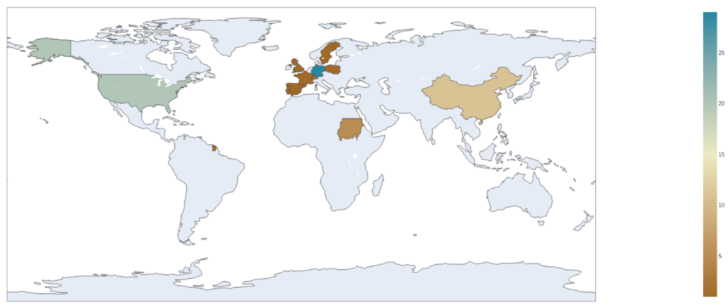
As you can see, rendering a world map using Plotly is fabulously easy, and the key here is to use a dictionary of choropleth type.
Now let’s try a slightly more complex example. This time we will visualize the relationship between countries. As in the previous example, the colors of the countries will be hardcoded. On the other hand, the relations connecting the countries will be loaded from a CSV file, which will store the relation’s weight and the geographical coordinates of its starting and ending points (note that in the general case, these do not have to be the center points of the individual countries).
Take a look at the snippet below:
import plotly.graph_objects as go
import pandas as pd

df_countries = pd.read_csv('./data/nodes.csv')
df_weights = pd.read_csv('./data/edges.csv')

for index, row in df_weights.iterrows():
    start = row["Source"]
    end = row["Target"]
    df_weights.at[index,"start_lon"] = df_countries.loc[df_countries["Id"] == start]["lng"].values[0]
    df_weights.at[index,"start_lat"] = df_countries.loc[df_countries["Id"] == start]["lat"].values[0]
    df_weights.at[index,"end_lon"] = df_countries.loc[df_countries["Id"] == end]["lng"].values[0]
    df_weights.at[index,"end_lat"] = df_countries.loc[df_countries["Id"] == end]["lat"].values[0]

fig = go.Figure()

data = dict (
    type = 'choropleth',
    locations = ['Argentina', ' Australia', ' Austria', ' Belgium', ' Botswana', ' Bulgaria', ' Chile', ' China', ' Czech Republic', ' Denmark', ' Ecuador', ' Finland', ' France', ' Germany', ' Ghana', ' Greece', ' Hungary', ' India', ' Indonesia', ' Ireland', ' Italy', ' Jamaica', ' Japan', ' Latvia', ' Lebanon', ' Lithuania', ' Malaysia', ' Mexico', ' Nepal', ' Netherlands', ' Nigeria', ' Norway', ' Poland', ' Romania', ' Russian Federation', ' Slovenia', ' South Africa', ' South Korea', ' Spain', ' Sweden', ' Switzerland', ' Tanzania', ' Thailand', ' Turkey', ' Uganda', ' Ukraine', ' United Kingdom', ' United States', ' Uruguay', ' Zimbabwe'],
    locationmode='country names',
    colorscale='portland',
    z=[1, 2, 1, 1, 1.066667, 1.333333, 0.733333, 5.666667, 0.666667, 1.833333, 1, 0.666667, 1, 4, 4.5, 4, 0.333333, 0.5, 1, 1, 3.666667, 0.5, 0.5, 0.4, 1, 0.333333, 1, 4, 1, 2, 1.5, 0.833333, 1.4, 0.333333, 0.666667, 1.333333, 6.5, 1.5, 2, 2.833333, 1.333333, 1, 1, 1, 1.5, 1.333333, 8.666667, 18.566667, 1, 1])

fig = go.Figure(data=[data])

fig.add_trace(go.Scattergeo(
    locationmode = 'country names',
    lon = df_countries['lng'],
    lat = df_countries['lat'],
    text = df_countries['Label'],
    showlegend = False,
    mode = 'markers'
    ))

for i in range(len(df_weights)):
    fig.add_trace(
        go.Scattergeo(
            lon = [df_weights['start_lon'][i], df_weights['end_lon'][i]],
            lat = [df_weights['start_lat'][i], df_weights['end_lat'][i]],
            mode = 'lines',
            showlegend = False,
            line = dict(width = 2 * df_weights["Weight"][i], color = 'lime'),
            opacity = 0.6
        )
    )

fig.update_layout(
    title_text = 'Sample map chart',
    showlegend = True,
    geo = dict(
        projection_type = 'natural earth',
        showland = True,
        landcolor = 'rgb(243, 243, 243)',
        countrycolor = 'rgb(204, 204, 204)',
    )
)

fig.update_geos(
    visible=False,
    showcountries=True, countrycolor="Black"
)

fig.show()
And this is the result we achieved:
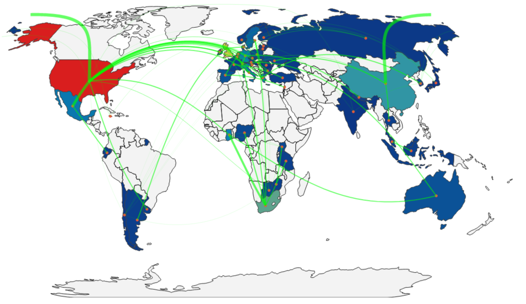
Doesn’t using the Plotly library produce truly beautiful results?